Introduction

Segmentation is the process of partitioning a digital image into multiple meaningful sections which is useful in many areas. There are many classical methods to implement image segmentation such as thresholding according to the image intensity, clustering and edge detection like Canny edge detecter.

While many segmentation methods rely heavily in some way on edge detection, the Chan-Vese model for active contours ignores edges completely[1]. The model is based on an energy minimization problem, which can be reformulated in the level set formulation, leading to an easier way to solve the problem. And it is based on Mumford-Shah functional for segmentation[2].

In this paper, we will also do some experiments on different images and different pair of parameters to test performance of this algorithm and talk about the strengths, weaknesses and potential future improvements.

The Chan-Vese Model

The Chan–Vese method is a region-based active contour method inspired by the Mumford–Shah model. It minimizes an energy which can be seen as a particular case of the minimal partition problem. As a result, we have to define an energy functional and at each time stamp, the goal of the Chan-Vese model is to progress to a lower energy which means it has to minimize the energy in both sides of the contour.

The energy functional used in Chan-Vese model can be defined as follows:

$$\begin{equation} E(C,u,v) = \lambda_1 \iint_R(I-u)^2dxdy + \lambda_2 \iint_{R^C}(I-u)^2dxdy + \mu \int_Cds + \nu \iint_Rdxdy \end{equation}$$

The energy functional is represented by four terms where $I$ denotes the image, $u$ and $v$ are the average intensity respectively inside and outside of the contour, $C$ is the contour, $R$ is the region inside of the contour and $R^C$ is the region outside of the contour. $\lambda_1, \lambda_2, \mu, \nu$ are fixed parameters which are chosen by us. The overall goal is to minimize all of the four terms at each time step. The first term is the energy inside of the contour and the second term is the energy outside of the contour. These two terms represent the discrepancy between the image $I$ and the two constants $u$ and $v$, to minimize these two terms, we want to keep the regions as uniform as possible. The third term penalize the length of the contour which will keep the contour as short and smooth as possible to avoid complicated curves and help us dealing with noisy situations. The fourth term penalize the enclosed area of the contour to control its size.

Algorithm in Pseudo Code

The basic implementation of the Chan-Vese model can be described as follows:

1. Initialize $\lambda_1, \lambda_2, \mu, \nu, \Delta t$.
2. Initialize $\psi^0$ with a desired shape and location for the contour.
3. Use the region defined by the current contour to compute the average intensity $\mu, \nu$.
4. Calculate $\psi_t$.
5. Calculate $\psi^{n+1} = \psi^n + \Delta t\cdot \psi_t$ to evolve contour.
6. Check whether the solution is stationary, if not, repeat step 3 - 5, else stop.

In this paper, in order to simplify the code, we set $\Delta x = \Delta y = 1$. Applying this to the CFL condition, we have $\Delta t \leq 0.5$. So we set $\Delta t = 0.1$. For the remaining parameters in step 1, we will first set the default value as $\lambda_1 = \lambda_2 = 1, \mu = 0.5, \nu = 0$. We will then discuss the results of choosing different pairs of parameters.

Experimental Results

Performance on Regular Images

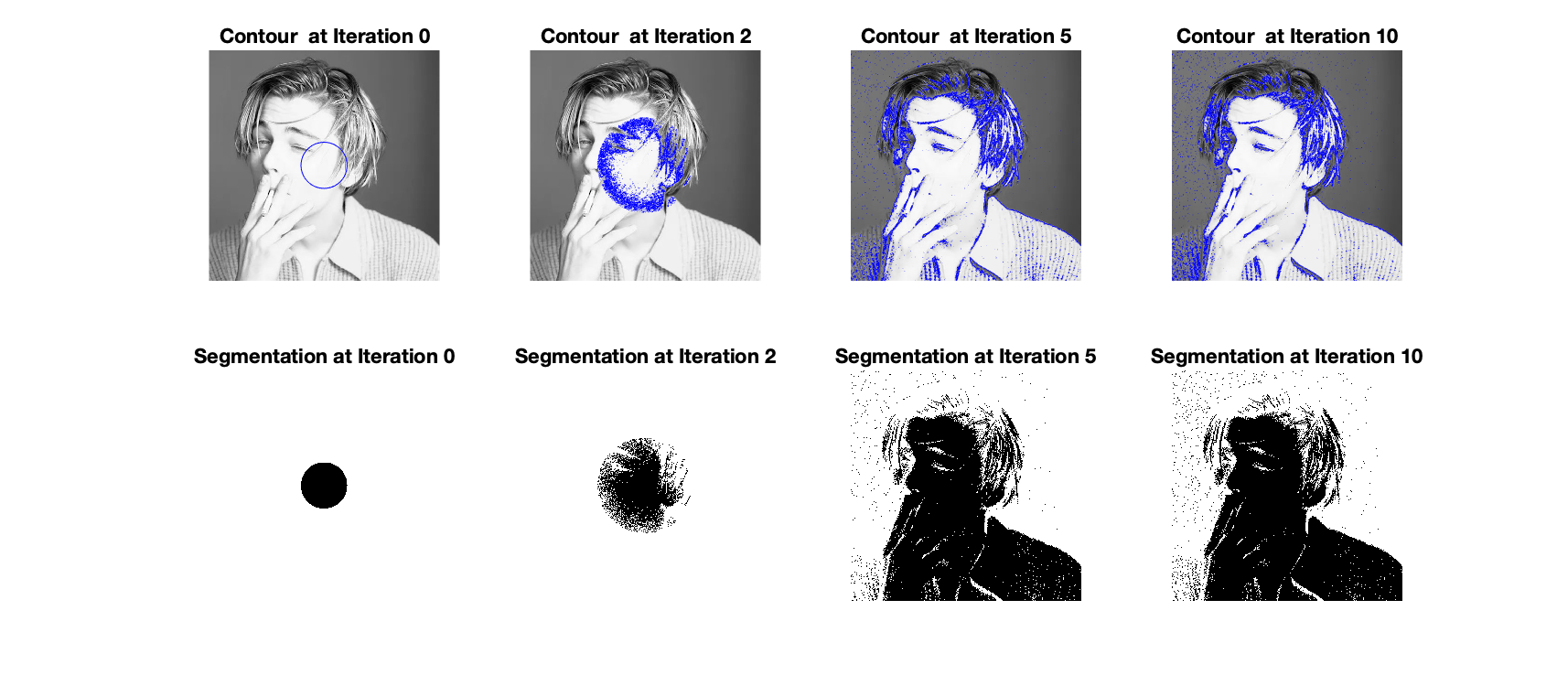
First, we applied the Chan-Vese model with default parameters to a picture of “Leonardo” and recorded the contour derived by each iteration as shown below.

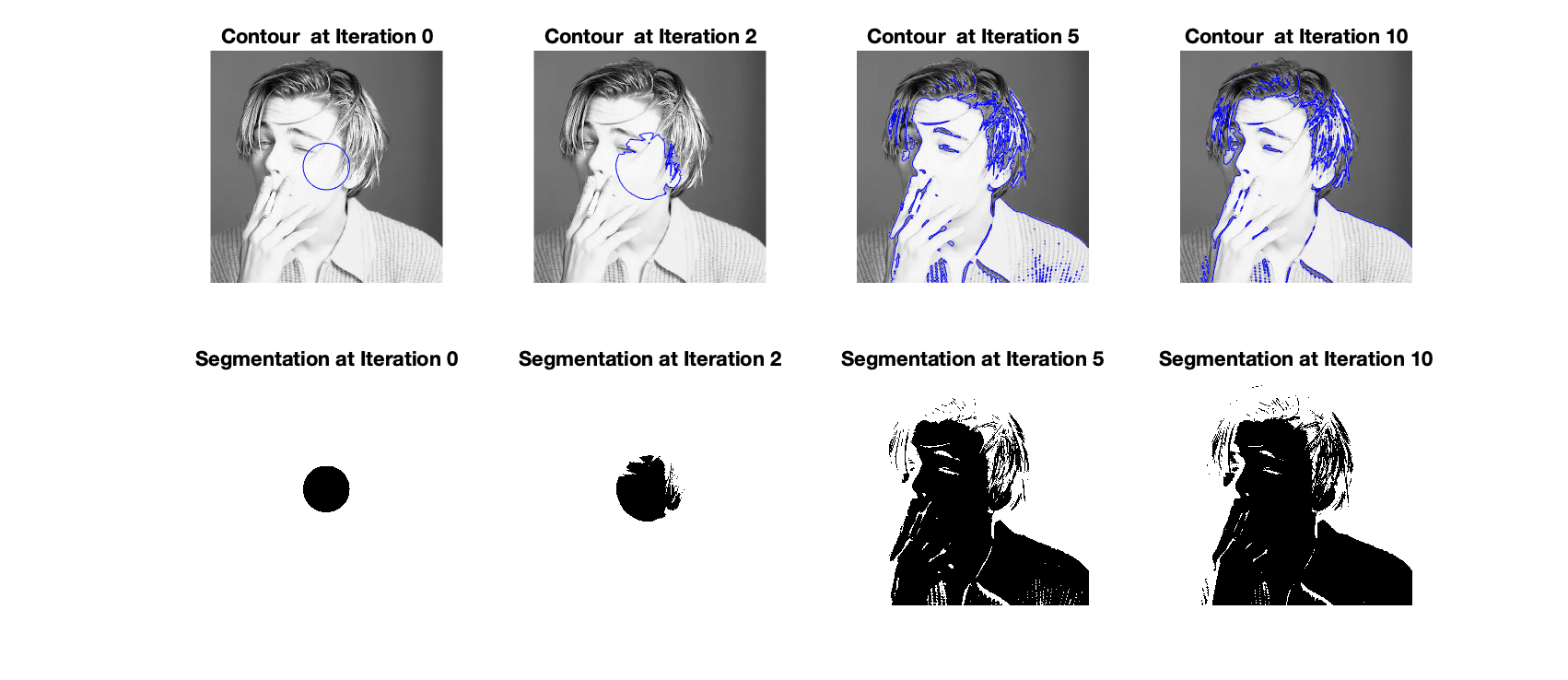
From the evolution of the contour, we can see that only after five iterations, we can obtain an overall contour of the image. And the result is quite good.

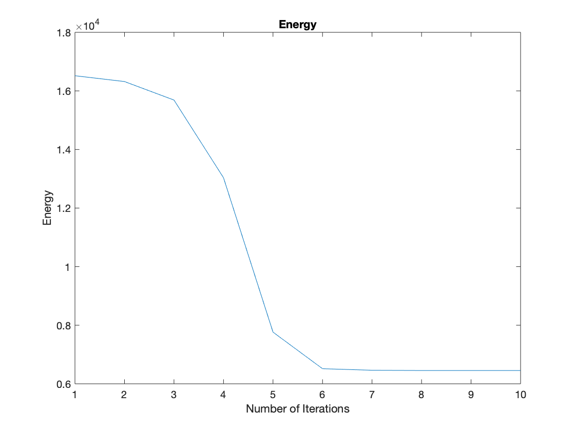
Since in Chan-Vese model, at each step, our goal is to minimize the energy funcitonal, we can further examine this model, we then look at the evolution of energy after each iteration. As shown below, we can see that there is a sharp drop between the third and fifth iterations which corresponds to the fully evolving of the contour, we can also see that after six rounds of iterations, the energy becomes stable.

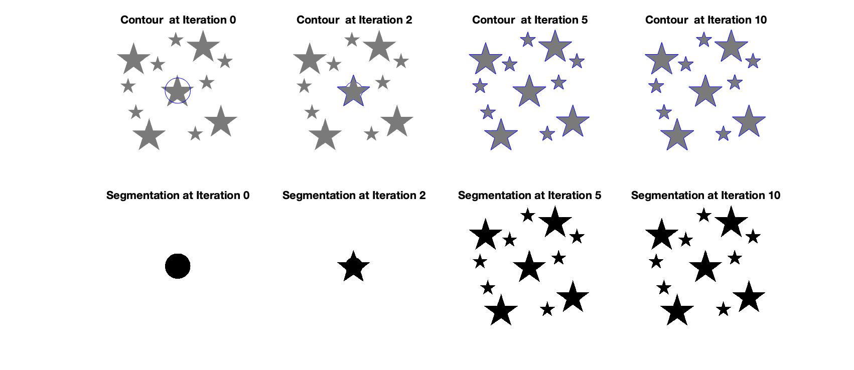
Now, let’s implement the Chan-Vese Algorithm on a texture picture of stars. As shown below, we can see that the Chan-Vese algorithm explicitly contour the edge of each stars which shows that this algorithm works best under the situation when the object can be clearly separated from the background.

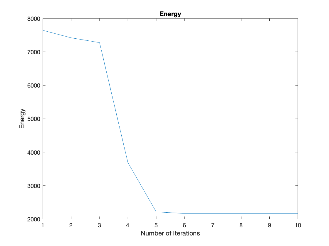
The energy evolution shown below also shows that Chan-Vese Algorithm can quickly reach the minimal of the energy.

Performance on Nosiy Images

In order to further test the practicality of this algorithm, we run some tests on noisy images, and here are the results. As shown below, we added Gaussian noise to the image “Leonardo”.

And Salt & Pepper noise to the image “Leonardo”.

We can see from the results that although there are some undesirable effects due to the noise, we can still obtain the overall contour of the image. We can also see that different kinds of noise have different impacts on this algorithm, when adding Salt & Pepper noise to the image, the final contour enclosed more noise pixels and the result is worse than adding Gaussian noise.

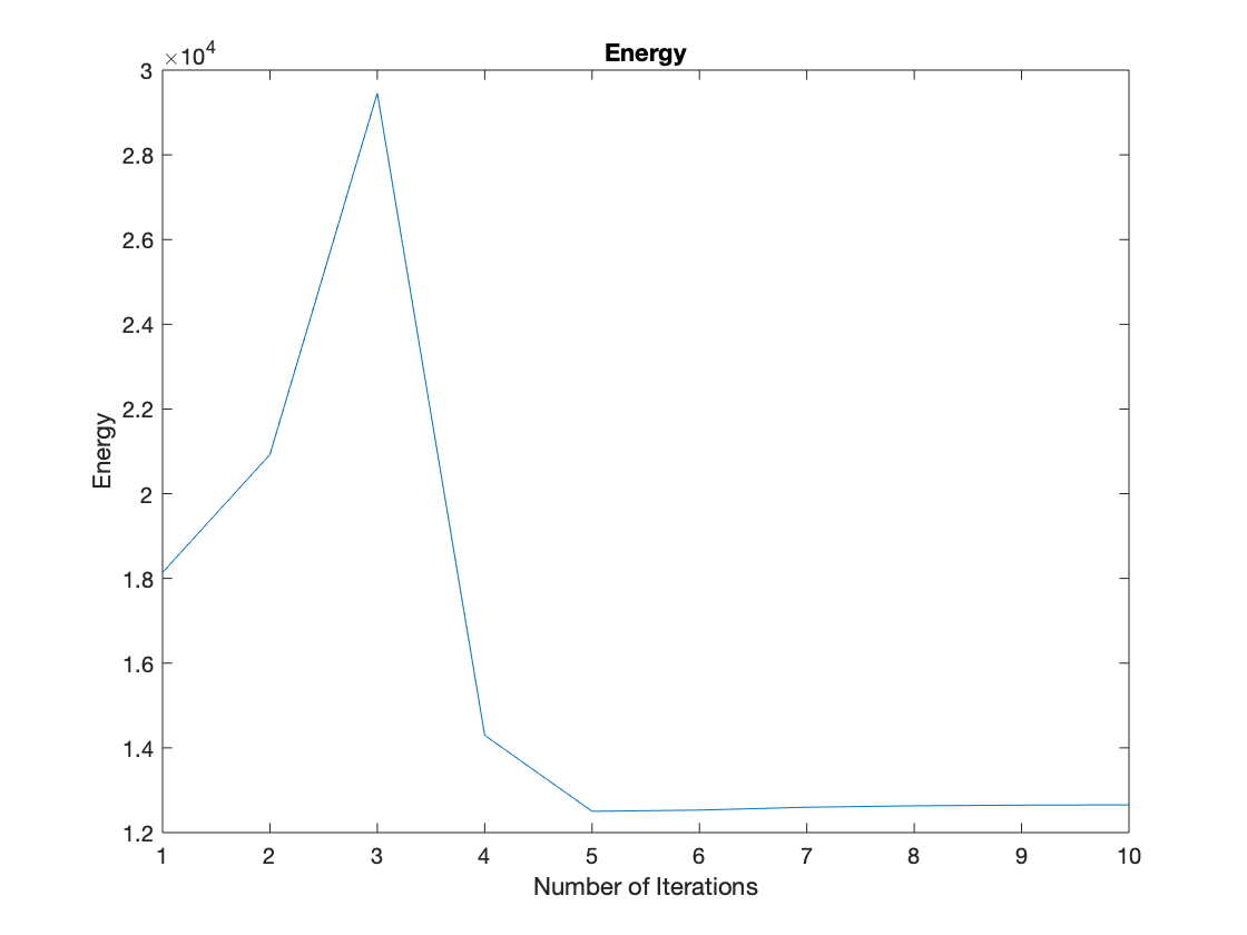
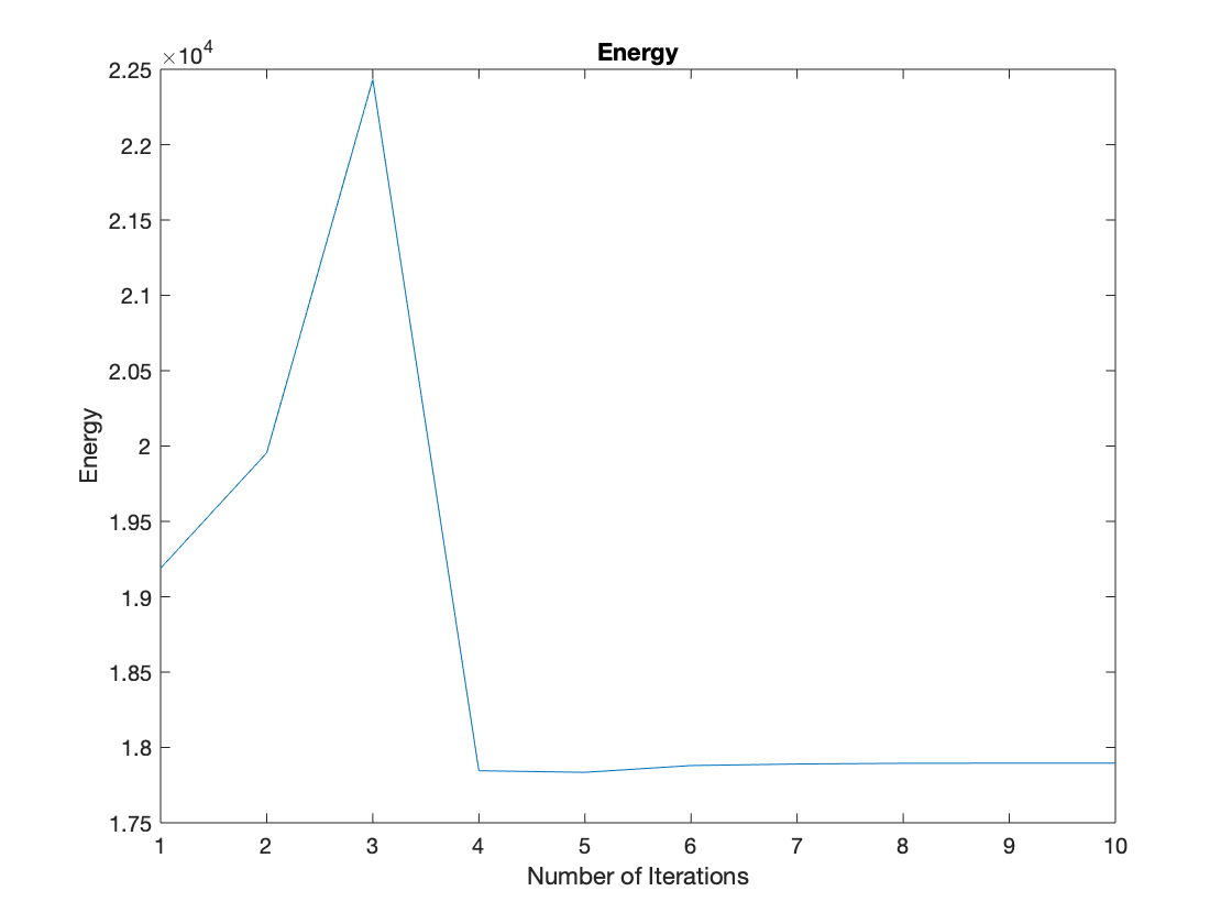
As for the energy evolution, different from the energy evolution of the regular picture, we can see that the energy first go up rapidly and then go down sharply before reaching a steady state due to noise pixels. The final minimal energy of “Leonardo” with Gaussian noise is also lower than “Leonardo” with Salt & Pepper noise.

Effect of Varying $\mu$

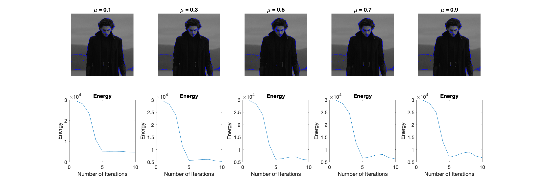
In Chan-Vese algorithm, parameter $\mu$ adjusts the length penalty, which balances between fitting the input image more accurately (smaller $\mu$) versus producing a smoother boundary (larger $\mu$) as shown below.

Effect of Varying $\nu$

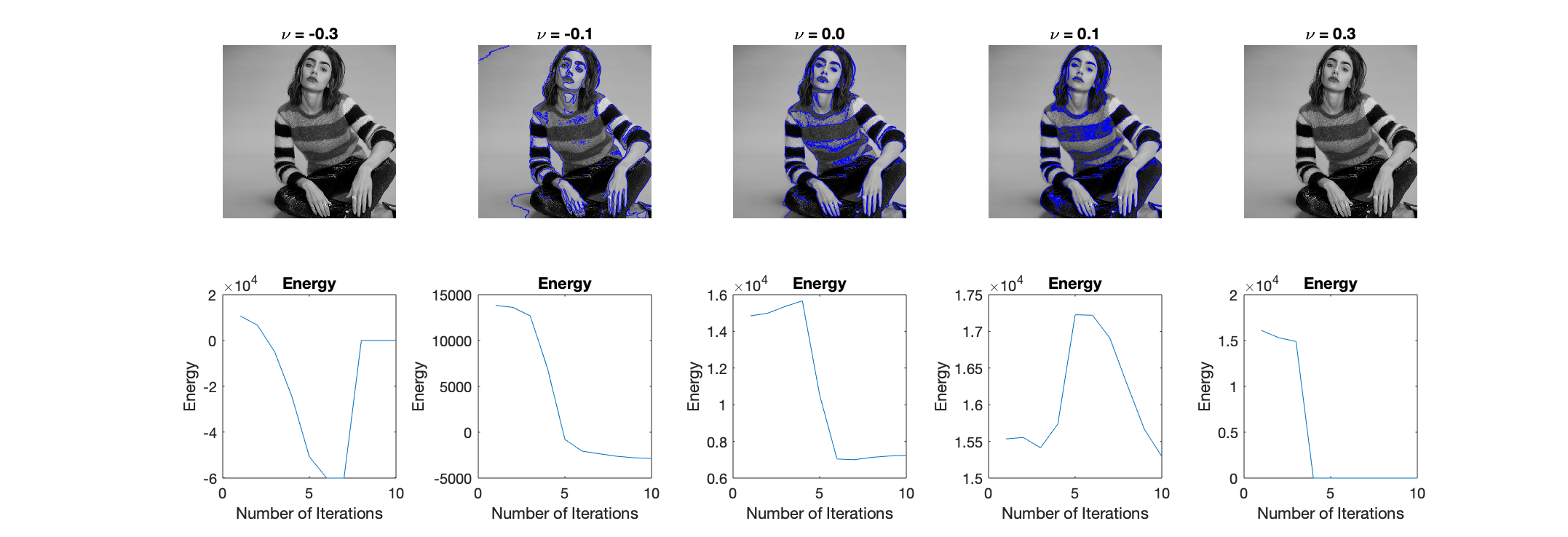
Parameter $nu$ sets the penalty (or reward, if $\nu < 0$) for area inside the contour. Noting that this parameter is meaningful only when there is a prescribed inside and outside of the segmentation boundary. In the figure below, the evolution is shown with five different values of $\nu$. When $\nu$ is too negative, the boundary expands to fill the full domain, and when $\nu$ is too positive, the boundary shrinks until it vanishes.

Effect of Varying Number of Initialization Curves

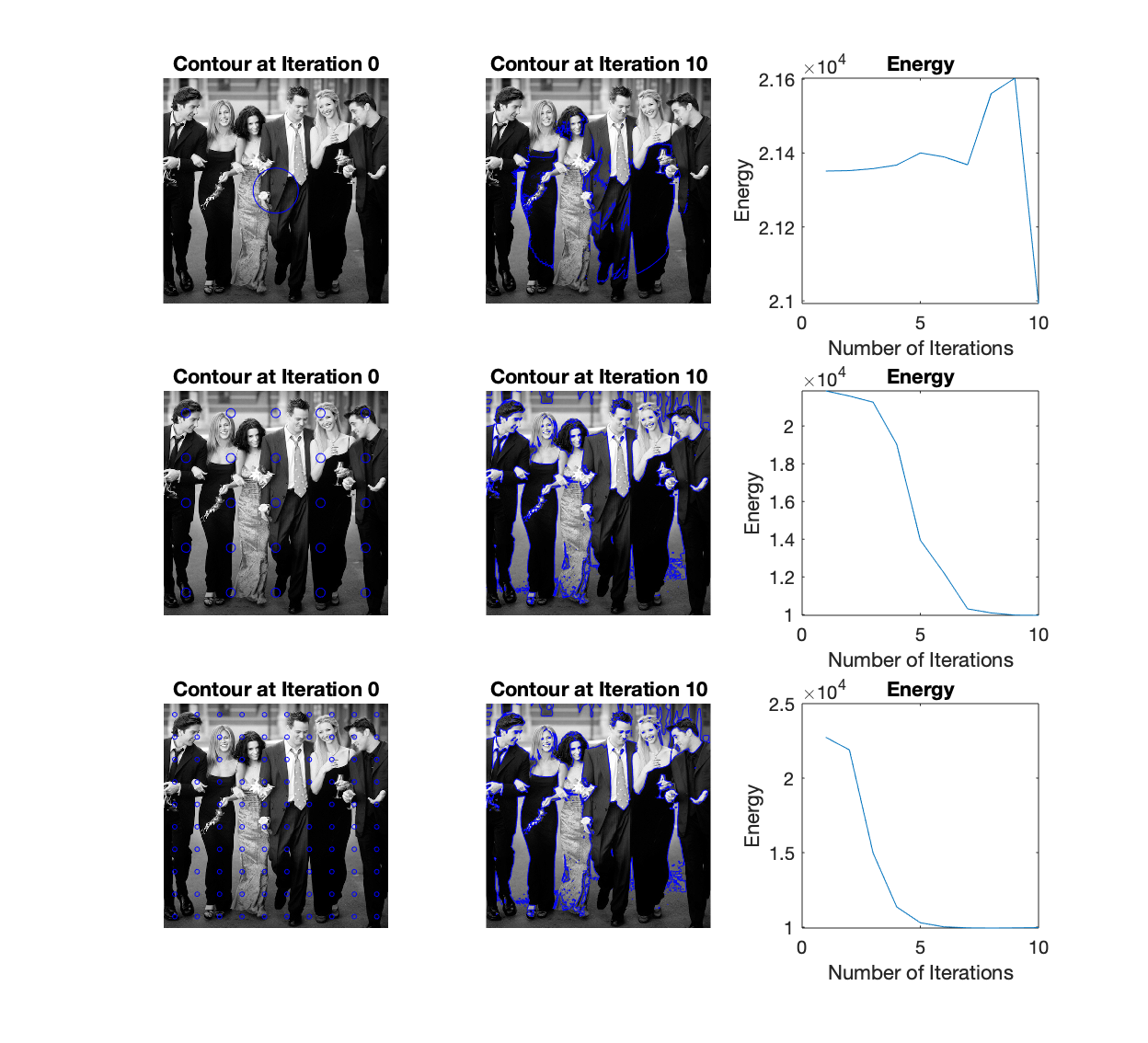
For above experiments, we only used a simple circular level-set for initialization, and in this section, we tested effects of different number of curves used for initialization as shown below. Although the final minimal tends to be the same after several iterations, the number of curves used for initialization has a great impact on the number of iterations needed to derive the contour.

Conclusions

Strengths and Weaknesses

Overall, the Chan-Vese algorithm seems to be a value tool in the area of image segmentation. It can quickly find the contour and it relies on global properties like intensities and region areas, rather than just taking into account local properties, such as gradients. However, this makes it difficult for the Chan-Vese algorithm to deal with noisy pictures. And, if we take the length of the contour and the region enclosed by the contour into consideration, these penalty or reward may have negative effects on the results which is not what we want in the first place.

Potential Improvements

Many implementations of the Chan-Vese algorithm including a reinitialization step since the Chan–Vese model generally has multiple local minimizers. By using an initial boundary, specific objects in the image can be segmented. And reinitialization may need to be used to avoid including separate objects and allow it to maintain a single closed curve.

Also, in order to refine the algorithm, some implementations use values that were already computed to decrease the computing time of the next values and reduce the time of computing PDE equations at each loop which my save a lot of time.

The Chan-Vese algorithm can also be used to segment color images which was not discussed in this paper.

So if there was more time, we will focus on the three problems above and try to do more experiments to test the performance of this algorithm on different kinds of images.

References

[1] T. F. Chan and L. A. Vese. Active contours without edges. IEEE Transactions on Image Processing, 10(2):266–277, 2001.

[2] David Mumford. Optimal approximation by piecewise smooth functions and associated varia- tional problems. Commun. Pure Applied Mathematics, pages 577–685, 1989.